|
Sinalgo - Simulator for Network Algorithms |
Sinalgo Tutorial
Sinalgo is a simulation framework for testing and validating network algorithms. Unlike most other network simulators, which spend most time simulating the different layers of the network stack, Sinalgo focuses on the verification of network algorithms, and abstracts from the underlying layers: It offers a message passing view of the network, which captures well the view of actual network devices. Sinalgo was designed, but is not limited to simulate wireless networks.
The key to successful development of network algorithms is a comprehensive test suite. Thanks to the fast algorithm prototyping in JAVA, Sinalgo offers itself as a first test environment, prior to deploy the algorithm to the hardware. Prototyping in JAVA instead of the hardware specific language is not only much faster and easier, but also simplifies debugging. Sinalgo offers a broad set of network conditions, under which you may test your algorithms. In addition, Sinalgo may be used as a stand-alone application to obtain simulation results in network algorithms research.
Sinalgo's view of network devices is close to the view of real hardware devices (e.g. in TinyOS): A node may send a message to a specific neighbor or all its neighbors, react to received messages, set timers to schedule actions in the future, and much more.
Some of the key features of Sinalgo:
Please refer to the Tutorial for more information on how to get started.
This software was developed by the Distributed Computing Group at ETH Zurich.
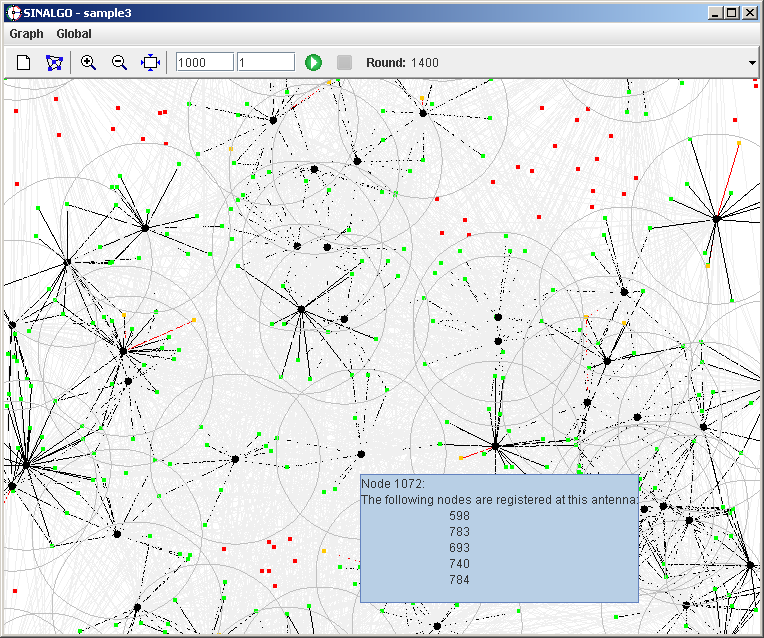

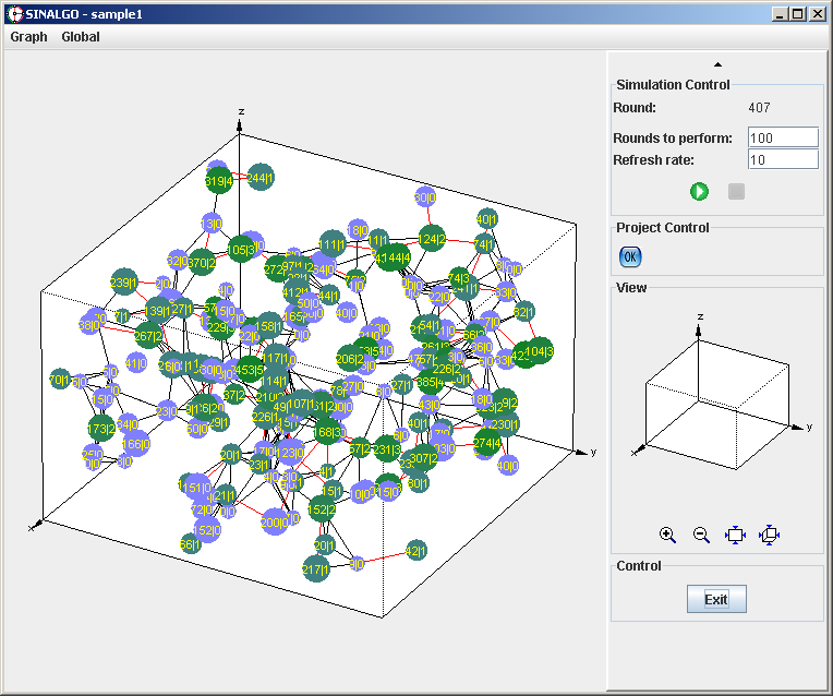
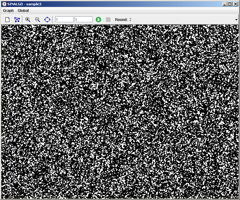
Screenshots
Running a simulation is actually quite easy. The real difficulty is to understand what one has simulated, and to interpret the obtained results in this context. With this in mind, we hope to give you enough information to not only understand how you can use this simulation framework, but also understand on a high level how the simulation executes. For this purpose, we have added a section Architecture that gives an insight into the clockwork of Sinalgo.
In case you have several versions of Java installed, ensure that the default version is 5.0 or higher.
Note: If another application than java executes jar files on your system, you may need to launch Sinalgo from the command line. This is probably the case if you see a window showing a directory structure after double clicking the jar file. To start Sinalgo from the command line, open the a command line and change to the unpacked directory of the toy release. Then, type java -jar sinalgo.jar
To run the application from the command line, call (for
example)
java -cp binaries/bin
sinalgo.Run
Refer to the Command Line Arguments section of the tutorial
for more information about the command-line arguments to Sinalgo.
To start the application, right-click on the src folder in the Package Explorer or the Navigator of Eclipse, and select 'Run As' -> 'Java Application'.
For Eclipse Users: In the Navigator or Package Explorer of Eclipse, open the folder src/sinalgo/. Right-click on Run.java and select Run As -> Java Application. (There are several alternatives to launch an application in Eclipse, please consult the documentation of Eclipse for more details.)
Note: Do not use the -Xmx flag for the virtual machine. This flag only affects the Run application, which starts the simulation in a separate process.
Depending on your OS and installed applications, you may have several tools at hand that may facilitate simulations with Sinalgo. Below is a brief list of how you may edit the javaCmd field in the config file:
| java | The default. Just start the simulation process. |
| nice -n XX java | Start Sinalgo with modified priority XX. |
| time java | Display the total running time of the simulation (after the simulation stopped). |
By passing on arguments on the command line (or through your IDE), you can influence the execution of Sinalgo. The following list describes the recognized command line arguments.
| -help | Prints the recognized command line arguments. |
| -gui | Starts the framework in GUI mode (default) |
| -batch | Starts the framework in batch mode, i.e. no windows. This mode is best suited to run long-lasting well-defined simulations. |
| -project XX | Indicates that Sinalgo should be started for project XX. If this argument is missing, the project selector dialog will be displayed. |
| -rounds XX | The framework performs XX simulation rounds immediately after startup. Defaults to zero. |
| -refreshRate XX | Sets that the GUI should be updated only every XX round. Defaults to 1. |
| -gen ... |
This argument lets you automatically generate network nodes. It has
the following form: -gen #n T D {(params)} {CIMR {(params)}}* The command generates #n nodes of node-type T and distributes them according to the distribution model D. (Optionally, the distribution model may take parameters in parentheses.) Optionally, you may specify in arbitrary order the connectivity, interference, mobility, and reliability models by appending the corresponding model name(*) to the -gen command. If a model is not specified, the default model (as specified in the project's configuration file) is used. (Again, any of the model names may be followed by model-specific arguments enclosed in parentheses.) (*) Model and Node Naming Convention: The name of models is composed of the project name in which the model is located and the name of the model itself: projectName:modelName. The same holds for the name of the node. Exception: Models and nodes stored in the defaultProject of the framework need not be prefixed with "defaultProject:". For disambiguation, the models may be prefixed with X=, where X={C|I|M|R}. The mapping is as following:
|
| -overwrite key=value (key=value)* | Overwrites the configuration entry named key to have the new value value. key may specify a framework configuration entry, or a custom configuration entry specified in the project's configuration file. |
-project sample1 -gen 1000 sample1:S1Node Random -rounds 10 -refreshRate 2
-project sample2 -gen 10000 sample2:S2Node Random C=QUDG M=sample2:LakeAvoid
Note that in this case, the disambiguation is not necessary, and the following arguments result in the same behavior.
-project sample2 -gen 10000 sample2:S2Node Random QUDG sample2:LakeAvoid
-overwrite mobility=true interference=false GeometricNodeCollection/rMax=50
-project sample1 -gen 100 sample1:S1Node Random UDG -gen 50 DummyNode Circle QUDG -gen 10 sample2:S2Node Random
Thus, it is possible to use nodes and models from several projects. But note that the configuration is loaded from the selected project.
-Djava.awt.headless=true
If you launch Sinalgo via the Run class, you may need to specify
this flag twice: once for calling Run, and once in the project
configuration through the javaCmd property.
Thanks to Denis Rochat for pointing out this issue.
only write:
|
#!/usr/bin/perl
$numRounds = 100; # number of rounds to perform per simulation for($numNodes=200; $numNodes<=500; $numNodes+=100) {
system("java -cp binaries/bin sinalgo.Run " .
}
"-project sample1 " . # choose the project
"-gen $numNodes sample1:S1Node Random RandomDirection " . # generate nodes "-overwrite " . # Overwrite configuration file parameters "exitAfter=true exitAfter/Rounds=$numRounds " . # number of rounds to perform & stop "exitOnTerminationInGUI=true " . # Close GUI when hasTerminated() returns true "AutoStart=true " . # Automatically start communication protocol "outputToConsole=false " . # Create a framework log-file for each run "extendedControl=false " . # Don't show the extended control in the GUI "-rounds $numRounds " . # Number of rounds to start simulation "-refreshRate 20"); # Don't draw GUI often |
The flags -project, -gen, -rounds, and -refreshRate are presented above. The remaining parameters overwrite the default entries in the project specific configuration file. Alternatively, we could add the flag -batch to run the simulation in batch mode. For huge simulations with many nodes, this may be preferable. But if memory is not a limiting factor, the GUI may provide a good interface to supervise the simulation. Setting the refresh rate to a fairly high value, the GUI does not use a significant amount of simulation time. Note that pressing the stop button, and then continuing a simulation is perfectly OK and does not change the simulation result.
Note: Project sample1 contains a more sophisticated run-script to demonstrate the possibilities of perl.
Remember: Depending on your platform, you may need to adjust the class path separator. In the example above, we used the semicolon. But for instance on Linux, the separator is a colon, and yet other separators may be used on other platforms.
Hint: Set the logToTimeDirectory such that log-files are not overwritten by a subsequent simulation. To collect simulation data from the different simulations, designate a log-file to which each simulation appends to. See Logging for more information.
Installing perl: You may obtain a copy of perl from www.perl.org. Alternatively, install Cygwin and include the perl package.
a) Start Sinalgo directly using the following slightly modified command line.
This launches the simulation process directly, but does not allow to specify the maximum memory to be used through the config file. The -Xmx800m flag indicates that the JVM may use at most 800 MB of memory, adjust the value to your needs.
b) Use remote debugging: Some java debuggers can be attached to a remote process (even running on a different machine). Remote debugging requires two steps.
b.1) First, modify the run command for the simulation process s.t. it can communicate with the debugger. I.e. set the javaCmd entry of the config file to
java -agentlib:jdwp=transport=dt_socket,address=localhost:8000,suspend=n,server=y
This configures the JVM to receive connections. You are free to choose any (unused) port number in the address-flag.
b.2) After starting the simulation, launch the debugger and attach it to the application. In Eclipse, call Run -> Debug... and create a new configuration for a Remote Java Application. Select the Connection Type to be Standard (Socket Attach), and the Connection Properties to match the address specified in the javaCmd.
Note: Hot code replace is only possible if the signature of the replaced class files remains the same. I.e. you may change the body of a method, but not the signature of the method. It is neither possible to add/remove methods or global variables.
The Graph menu provides the following tasks:
Generate Nodes

|
Opens a dialog that adds new nodes to the simulation. You can specify the number of nodes to add, their initial distribution, as well as the node specific models. |
Clear Graph

|
Removes all nodes from the simulation. |
| Reevaluate Connections | Loops over all nodes and determines for each node the set of neighbor nodes, according to the node's connectivity model. This function is especially useful in the asynchronous simulation mode, where the connections are not updated automatically. |
| Infos | Prints some information about the current network graph, including the number of nodes and the number of (unidirectional) edges. |
| Export |
Creates a vector graphic image of the current view of the network graph and
writes it to an EPS or PDF file.
To output the graphic in PDF format, your machine needs to provide a tool that can convert from EPS to PDF. By default, the framework calls the epstopdf application. Change the field epsToPdfCommand in the framework section of the configuration file to specify a different application. |
| Preferences | Some preferences you are allowed to change at runtime. This includes the type of the edges and the message transmission model, which is the same for all nodes. |
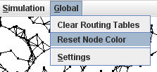
The Global menu contains all global custom methods and the Settings dialog, which displays a list of all settings.
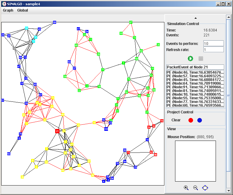
| Perform a simulation step / execute the next event |
Press the  button. In
synchronous simulation mode, this executes the number of rounds
specified in the Rounds to Perform text field. In asynchronous
simulation mode, this executes the number of events specified in the
Events to Perform text field. button. In
synchronous simulation mode, this executes the number of rounds
specified in the Rounds to Perform text field. In asynchronous
simulation mode, this executes the number of events specified in the
Events to Perform text field.
|
| Abort a running simulation |
Press the  button. After pressing the button, the simulation will finish the
currently executing round/event before it stops. Thus, this button is
only useful if you set the Rounds to Perform or Events to
Perform field to a value above 1.
button. After pressing the button, the simulation will finish the
currently executing round/event before it stops. Thus, this button is
only useful if you set the Rounds to Perform or Events to
Perform field to a value above 1.
The framework finishes the current round/event to ensure integrity of
the system, and that the simulation can be continued by pressing |
| Add an edge from node A to node B. | Left-click on node A. Keep the mouse pressed, move it to node B and release it. |
| Move a node in in 2D | Right-click on the node and drag it to the new place. Alternatively, right-click on the node to obtain the popup menu for the node and select the 'Info' dialog to key in the new coordinates. The latter approach is also supported in 3D. |
| Zoom in / Zoom out |
Position the mouse in the area containing the network and use the
wheel to change the zoom factor. Alternatively, use the zoom-in /
zoom-out buttons   . .
This operation may also be performed in the 'View' panel of the extended control panel. |
| Zoom to Fit |
Press the  button to set the
zoom factor such that the simulation area just fits on the screen. button to set the
zoom factor such that the simulation area just fits on the screen.
In 3D mode, press the |
| Translate the displayed simulation area |
Press the right mouse-button on a free spot of the simulation
area. Keep the mouse button pressed and move the mouse to translate
the simulation area.
This operation may also be performed in the 'View' panel of the extended control panel, with the difference that the network graph is only updated once the mouse button is released. This may be handy for huge networks graphs with a long drawing time. |
| Rotate the 3D cube |
Press the left mouse-button on a free spot of the simulation
area. Keep the mouse button pressed and move the mouse to rotate the
simulation area. By default, the rotation keeps the Z-axis
vertical. To turn off this feature, press the Ctrl button while pressing the left mouse-button.
This operation may also be performed in the 'View' panel of the extended control panel, with the difference that the network graph is only updated once the mouse button is released. This may be handy for huge networks graphs with a long drawing time. |
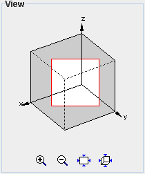
| The view panel in the extended control shows the entire cube even though the main view of the network graph only shows a cut-out. The red rectangle indicates the portion of the simulation area currently displayed. The zoom, translate and rotate operations may also be performed in this area. |
|
Note: It is recommended to generate a project for each algorithm one simulates. However, this often results in quite a lot of common code, e.g. models that are used for several projects. Instead of copying this code to all projects, it is preferred to create a dummy project that holds this common code from where all other projects access it. In fact, the defaultProject shipped with Sinalgo is such a dummy project and gathers quite some default implementations that may be handy for you.
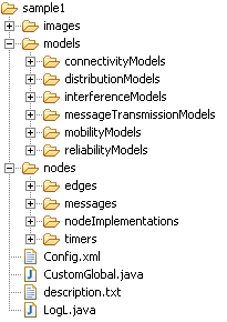
Each project contains the four following files in the root directory:
As in reality, the nodes implement their own behavior. Among others, they have a method that is called when the node receives a message, and they implement the functionality to send messages to neighboring nodes. Depending on the simulation mode, the node's methods are called in a slightly different way. The following shows a high-level picture of the calling-sequences of the synchronous and asynchronous mode, which are described in more detail in the Architecture section of this tutorial.
Remember that mobility is not possible in the asynchronous mode. However, the messages may be checked for interference if interference is turned on in the configuration file.
The following list gives the most useful members of the sinalgo.nodes.Node class you may use. For a complete description of their functionality, refer to the documentation in the code.
| Public Member Variables | |
| int ID | Each node is assigned a unique ID when it is created. This ID may be used to distinguish the nodes. |
| Connections outgoingConnections; | A collection of all edges outgoing from this node. Note that all edges are directed, the bidirectional edges just ensure that there is an edge in both directions. |
| Methods | |
| void send(Message m, int target) throws NoConnectionException; | Sends a message to a neighbor node with the default intensity of the node. |
| void send(Message m, int target, double intensity) throws NoConnectionException; | Sends a message to a neighbor node with the given intensity. |
| void send(Message m, Node target) throws NoConnectionException; | Sends a message to a neighbor node with the default intensity of the node. |
| void send(Message m, Node target, double intensity) throws NoConnectionException; | Sends a message to a neighbor node with the given intensity. |
| void sendDirect(Message msg, Node target); | Sends a message to any node in the network, independent of whether there is a connection between the two nodes or not. |
| void broadcast(Message m); | Broadcasts a message to all neighboring nodes with the default intensity of the node. |
| void broadcast(Message m, double intensity); | Broadcasts a message to all neighboring nodes with the given intensity. |
| Position getPosition(); | Returns the current position of the node. |
| TimerCollection getTimers(); | Returns a collection of all timers currently active at the node. |
| void setRadioIntensity(double i); | Sets the radio intensity of the node. |
| double getRadioIntensity(); | Gets the radio intensity of the node. |
| void setColor(Color c); | Sets the color in which the node is painted on the GUI. |
| Color getColor(); | Gets the color in which the node is painted on the GUI. |
| void draw(...); | Implements how the node is drawn on the GUI. You may overwrite this method in your subclass of sinalgo.node.Node to define a customized drawing. |
| void drawAsDisk(..., int sizeInPixels); | A helper method provided by sinalgo.node.Node that draws the node as a disk. Call this method in your draw(...) method. |
| void drawNodeWithText(..., String text, int fontSize, Color textColor); | A helper method provided by sinalgo.node.Node that draws the node as a disk and with text. Call this method in your draw(...) method. |
| void drawToPostScript(...); | Implements how the node is exported to PostScript. You may overwrite this method in your subclass of sinalgo.node.Node to define a customized drawing to PostScript. |
To control the creation of a node object, the super-class provides
the two methods init() and checkRequirements() which you may overwrite in
your subclass:
Node.init() is called once at the
beginning of the lifecycle of a node object. It may be used to
initialize the start state of the node. Note that this function may
not depend on the neighborhood of the node as the init function is
called before the connections are set up and before the set of all
nodes is available.
Node.checkRequirements() is called
after the init() method to check whether all requirements to use this
node type are met. This may include a test whether appropriate models
have been selected.
|
The annotation @NodePopupMethod(menuText="XXX") in the following
code sample declares the method myPopupMenu() to be included in the popup menu
with the menu text XXX. Note that the
methods to register with the popup menu may not take any parameters
and need to be located in the source-file of the specific Node subclass.
@NodePopupMethod(menuText="Multicast 2")
public void myPopupMethod() { IntMessage msg = new IntMessage(2);
}
MessageTimer timer = new MessageTimer(msg); timer.startRelative(1, this); |
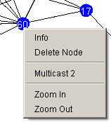
Customized node popup menu |
The sample code generates a message carrying an int-value, and broadcasts it to all its neighbors. Note that the method does not broadcast the message directly, but creates a timer, which will be triggered in the next round when the node performs its step. This is necessary for the synchronous simulation mode, because nodes are only allowed to send messages while they are executing their step. However, the user can only interact with the GUI while the simulation is not running. Therefore, the methods called through the popup menu always execute when the simulation is stopped. The preferred solution is to create a timer which fires in the next round and performs the desired action.
Note: The MessageTimer is available in the defaultProject. This timer may send a unicast message to a given node, or multicast a message to all immediate neighbors. Please consult the documentation of the source code for more details.
In some cases, it may be desirable to determine only at runtime the set of methods to be included in the menu, and on their menu text. This is possible because the popup menu for the node is assembled every time the user right-clicks on a node. The framework includes all methods annotated with the NodePopupMenu annotation of the corresponding node class. But before including such a method in the list, the framework calls the node-method includeMethodInPopupMenu(Method m, String defaultText), which allows to decide at runtime whether the menu should be included or not, and, change the menu text if necessary.
To obtain control over the included menu entries, overwrite the includeMethodInPopupMenu(Method m, String defaultText) method in your node subclass. Return null if the method should not be included, otherwise the menu text to be displayed.
The abstract class Message requires you
to implement a single method that returns a clone of the message,
i.e. an exact copy of the message object:
public Message clone()
Implementation Note: When a node sends a message to a neighbor node, it is assumed that the destination receives the message-content that was sent through the send() method. The framework has however no means to test whether the sender still has a reference to the sent message-object, and therefore may be able to alter its content. To avoid such problems, the framework sends separate copies to all receivers of a send() or multicast() call. Thus, for a multicast to n neighbors, the framework obtains n copies of the message and sends a copy to each of the neighbors.
If and only if your project ensures that a message-object
is not altered after it was sent, you may omit the copying process by
providing the following implementation of the clone() method. (Note that the process of sending
or receiving a message does not alter the message-object. Thus, a
node may safely forward the same message-object it has received.)
For each received message, this iterator stores meta-information, such as the sender of the message. This meta-information is available for the packet that was last returned through the next() method.
In order to iterate several times over the set of packets, you may reset the inbox by calling reset(), size() returns the number of messages in the inbox. Call remove() to remove the message from the inbox that was returned by the last call to next().
Typically, a node iterates over all messages in the inbox with the following code:
In asynchronous simulation mode, messages are kept in message-events, which are scheduled to execute when the message is supposed to arrive. At the time of execution, the framework decides whether the message arrives. If the message arrives, the method handleMessages() is called on the receiver node. If the message does not arrive, the method handleNAckMessages() is called on the sender node.
In synchronous simulation mode, a sender node can handle the set of messages that were scheduled to arrive in the previous round, but were dropped. The method handleNAckMessages() is called prior to handling the messages that arrive on the node, and passes on the set of dropped messages.
The use of the NackBox object, which holds the set of dropped messages, is equivalent to the Inbox.
A typical implementation of the handleNAckMessages(), which needs to be added to your node implementation if you want to use this feature, looks as following:
Note: The framework only supports one edge type at any time. The type to use can be specified in the configuration file, and it may be switched at runtime through the Preferences menu. Changing the edge type at runtime only affects edges created after the change. It does not replace the already existing edges.
The following edges are already available:
| sinalgo.nodes.edges.Edge |
The default edge implementation, superclass of all edges. This edge
is directional. As a result, Sinalgo does not really support
bidirectional edges in the sense that there is a single object for a
bidirectional edge. The bidirectional edge implementation solves this problem
by adding an edge in both directions.
By default, this edge draws itself as a black line between the two end-nodes, and colors itself red when a message is sent over the edge. |
| sinalgo.nodes.edges.BidirectionalEdge |
The default bidirectional edge implementation. It ensures that there is an edge
in both directions between the two end nodes.
By default, this edge draws itself as a black line between the two end-nodes, and colors itself red when a message is sent over the edge. |
|
projects.defaultProject.nodes .edges.BooleanEdge |
The BooleanEdge extends the default edge implementation with a
boolean member flag that may be used
arbitrarily. It also carries a static member onlyUseFlagedEdges, which may be used to enable
or disable globally the use of the flag.
The provided implementation uses onlyUseFlagedEdges and flag to decide whether the edge is drawn or not: If onlyUseFlagedEdges is true, the edge only draws itself if flag is set to true. |
|
projects.defaultProject.nodes .edges.BidirectionalBooleanEdge |
A bidirectional edge with the features of the boolean edge. |
|
projects.defaultProject.nodes .edges.GreenEdge |
The same as the default edge implementation, but it draws itself as a green line between the two end-nodes. |
To write a project specific timer, implement a subclass of sinalgo.nodes.timers.Timer and put the source file in the nodes/timers/ folder of your project. A timer instance is started by calling either the startAbsolute(double absoluteTime, Node n) method or the startRelative(double relativeTime, Node n) method of the super class. The time specifies when the task should be scheduled, and the node specifies the node on which the task should be executed.
Hint: The default project provides a MessageTimer that schedules to send a message at a given time. The message may be unicast to a specified recipient, or multicast to all immediate neighbors.
To create a global timer, implement a subclass of sinalgo.nodes.timers.Timer just as for the regular node timers. But in contrast to the node related timers, start the timer with its method startGlobalTimer(double relativeTime).
Hint: You may use the same timer implementation as a node-related timer and as a global timer. Just make sure that the fire() method of the timer class does not access the node member when the timer was started as a global timer. This member is set only when the timer is started as a node-related timer.
| customPaint(...) | This paint method is called after the network graph has been drawn. It allows for customizing the drawing of the graph by painting additional information onto the graphics. |
| handleEmptyEventQueue() |
The framework calls this method when running in asynchronous mode and
there is no event left in the queue. You may generate new events in
this method to keep the simulation going.
Note that the batch mode terminates when the event queue is emptied and this method does not insert any new events. |
| preRun() | Called once prior to starting the first round in synchronous mode, or prior to executing the first event in asynchronous mode. Use this method to initialize the simulation. |
| onExit() | Called by the framework before shutting down. To ensure that this method is called in all cases, you should use sinalgo.tools.Tools.exit() to exit, instead of System.exit(). |
| preRound() | Called in synchronous mode prior to every round. This method may be suited to perform statistics and write log-files. |
| postRound() | Called in synchronous mode after every round. This method may be suited to perform statistics and write log-files. |
| checkProjectRequirements() | The framework calls this method at startup after having selected a project to check whether the necessary requirements for this project are given. For algorithms that only work correctly in synchronous mode this method check that the user didn't try to execute it in asynchronous mode. If the requirements are not met, you may call sinalgo.tools.Tools.fatalError(String msg) to terminate the application with a fatal error. |
| nodeAddedEvent(Node n) |
Called by the framework whenever a node is added to the
framework (which is done through the method Runtime.addNode(Node n)).
This event may be useful for applications that need to update
some graph properties whenever a new node is added (e.g. by the user
through the GUI).
Note that this method is also called individually for each node created through the -gen command-line tool, and when the user creates nodes using the GUI menu. |
| nodeRemovedEvent(Node n) |
Called by the framework whenever a node is removed from the
framework (which is done through the method Runtime.removeNode(Node n)).
This event may be useful for applications that need to update
some graph properties whenever a node is removed (e.g. by the user
through the GUI).
Note that this method is not called when the user removes all nodes using the Runtime.clearAllNodes() method. |
Hint: The onExit() method may be a good place to perform final logging steps and project specific cleanup.
1) Drop Down Menu Entry: Prefix the method with the annotation
@AbstractCustomGlobal.GlobalMethod and
specify the menuText. E.g.
2) Icon Button: Prefix the method with the annotation @AbstractCustomGlobal.CustomButton and specify
the imageName and toolTipText. The imageName should be the name of a gif image of size 21x21 pixels, located in the
images folder of the project.
E.g.
3) Text Button: Prefix the method with the annotation @AbstractCustomGlobal.CustomButton and specify
the buttonText and toolTipText. E.g.
Project specific menu |
Project specific buttons |
The drop down menu entries (but not the buttons) may be adapted at runtime: Every time the user opens the 'Global' menu, the menu is assembled and includes methods annotated with the GlobalMethod annotation. Before including such a method in the list, the framework calls AbstractCustomGlobal.includeGlobalMethodInMenu(Method m, String defaultText) to allow the project to decide at runtime whether the method should be included or not, and, if necessary, change the default menu text.
Overwrite the method includeGlobalMethodInMenu(Method m, String defaultText) in your project specific CustomGlobal.java file to control the appearance of the 'Global' menu at runtime. The method returns the text to be displayed for each method, or null if the method should not be included.
In synchronous simulation mode, each node updates its connections
in every round. Refer to the synchronous
calling sequence section of this tutorial for more details. For
the asynchronous simulation, the framework does not support mobile
nodes. As a result, the framework does not call the connectivity
model at all, as it is often only necessary to setup the edges once
after the nodes have been created. Thus, the project is responsible
to call the following method at an appropriate time:
sinalgo.tools.Tools.reevaluateConnections();
This method calls the updateConnections(Node n) method on all nodes.
To facilitate the implementation of a new connectivity model, you
may create a subclass of sinalgo.models.ConnectivityModelHelper. This
helper class implements the updateConnections(Node
n) method, and asks the subclass to implement the method
boolean isConnected(Node from,
Node to);
which is often easier to implement.
The ConnectivityModelHelper assumes that the connectivity is geometric. I.e. there is a maximum distance between connected nodes, above which no node pair is connected. This assumption permits to drastically cut down the neighbor-nodes the helper class needs to test. Note that this maximum distance needs to be specified for each project. Refer to the configuration and architecture section of this tutorial to learn more about how to configure a project and how the geometric node collection stores the nodes to perform range queries for neighbor nodes.
For your convenience, the defaultProject already contains the following connectivity models. Note that these models are written as generic as possible. Therefore, you may need to add configuration settings to your project, depending on which model you select.
| UDG | The Unit Disk Graph connectivity is a purely geometric connectivity model: Two nodes are within communication range iff their mutual distance is below a given threshold. The maximal transmission radius, rMax needs to be specified in the configuration file of the project with an entry of the form <UDG rMax="..."/>. |
| QUDG | The Quasi Unit Disk Graph is similar to the UDG model, but does not have a sharp upper bound on the transmission range. In the QUDG model, a pair of nodes is always connected if their mutual distance is below a certain value rMin, and is never connected if their distance is above rMax. If the distance is between rMin and rMax, the nodes are connected with a certain probability, which has to be specified in the project configuration. See the source documentation of the QUDG class for more details. |
| StaticUDG | The static UDG model is the same as the UDG model, but it it evaluates the connections only the very first time it is called. This may be beneficial for projects where nodes do not move, and the connectivity does not change over time. |
| StaticConnectivity | The static connectivity model does not change the edges of a node at all. This model may be useful if the project has other means to generate and update the edges between neighboring nodes. |
The model requires to implement the method boolean isDisturbed(Packet p), which tests, whether a message arriving at this node may be disturbed by interference.
Implementation Notes: The Packet object passed to the isDisturbed(Packet p) method holds the message, the sender and receiver node, the intensity at which the sender is sending this packet, and other information that may be useful. To obtain a collection of all messages being sent at this moment, call sinalgo.tools.Tools.getPacketsInTheAir().
In synchronous simulation mode, the framework performs the interference test in every round. Refer to the synchronous calling sequence section of this tutorial for more details. For asynchronous simulations, the interference test is performed whenever an additional message is being sent or a message arrived.
Additive interference in asynchronous mode: By default, the
asynchronous mode performs an interference test on all messages that
have not yet arrived whenever an additional message is sent, or a
message arrives. This is a quite expensive operation, and is not
necessary in most cases, where the interference is
additive. We call interference additive, if
a) an additional message can only increase (or not
alter) the interference at any other receiver node, and
b) the interference decreases (or remains
the same) if any of the messages is not considered.
If all used interference models are additive, the framework
can reduce the calls to the interference test drastically. Additive
interference can be enabled/disabled in the configuration file of the
project.
For your convenience, the defaultProject already contains the following interference models. Note that these models are written as generic as possible. Therefore, you may need to add configuration settings to your project, depending on which model you select.
| SINR |
The signal to interference model is probably the best known
interference model. It determines a quotient q = s / (i+n) between
the received signal s and the sum of the ambient background noise n and
the interference i caused by all concurrent transmissions. The
transmission succeeds if q > beta, where beta is a small constant.
This model assumes that the intensity of an electric signal decays exponentially with the distance from the sender. This decrease is parameterized by the path-loss exponent alpha: Intensity(r) = sendPower/r^alpha. The value of alpha is often chosen in the range between 2 and 6. To the interference caused by concurrent transmissions, we add an ambient noise level N. This model requires the following entry in the configuration file: <SINR alpha="..." beta="..." noise="..."/> where alpha, beta, and noise are floating point values. |
| NoInterference | A dummy interference model that does not drop any messages due to interference. When using this model for all nodes, you should turn off the support for interference in the project configuration. |
The model requires to implement the method Position getNextPos(Node n), which returns the new position of node n.
In Sinalgo, mobility is simulated in terms of rounds. At the beginning of each round, the nodes are allowed to move to a new position, where they remain for the remainder of the round. (Refer to the calling sequence for more details.)
Implementation Note: The discretization of the movement may be refined in the following way: Assume a simulation, where nodes move 1 distance unit per round. At the same time, a message takes 1 round to arrive at its destination. To achieve a higher resolution of the movement, you may reduce the node speed to 0.1 distance units per round, and increase the message transmission time to 10. Along this line, you may achieve arbitrarily close approximations to a continuous system, paying with simulation time.
For your convenience, the defaultProject already contains the following mobility models. Note that these models are written as generic as possible. Therefore, you may need to add configuration settings to your project, depending on which model you select.
| RandomWayPoint |
A node that moves according to the random way point mobility model
moves on a straight line to a (uniformly and randomly selected)
position in the deployment field. Once arrived, it waits for a
predefined amount of time, before it selects a new position to walk
to.
The node speed and waiting time have to be configured through the project configuration. Both of them are defined through distributions. An entry in the configuration file may look as following:
<RandomWayPoint>
<Speed distribution="Gaussian" mean="10" variance="20" />
</RandomWayPoint>
<WaitingTime distribution="Poisson" lambda="10" /> Note: The stationary distribution of nodes moving according to the random way point model is not uniformly distributed. The nodes tend to be more often around the center of the deployment area than close to the boundary. |
| RandomDirection |
Similarly to the random way point model, the random direction model
alternates between waiting and moving periods. The only difference is
the choice of the target: Instead of picking a random point from the
deployment field, the random direction chooses a direction in which
the node should walk, and how long the node should walk in this
direction. If the node hits the boundary of the deployment area, it
is reflected just as a billard ball.
The node speed, move-time, and waiting time have to be configured through the project configuration and are defined through distributions. An entry in the configuration file may look as following:
<RandomDirection>
<NodeSpeed distribution="Constant" constant="0.4" />
</RandomDirection>
<WaitingTime distribution="Exponential" lambda="10" /> <MoveTime distribution="Uniform" min="5" max="20" /> Note: The stationary distribution of nodes moving according to the random direction model is uniformly distributed. |
| NoMobility | A dummy mobility model that does not move the nodes. When using this model for all nodes, you should turn off the support for mobility in the project configuration. |
The model requires to implement the method boolean reachesDestination(Packet p), which determines whether the message arrives at the destination or not. Note that the interference model may overrule this decision and drop a message due to interference. However, the interference model cannot reincarnate an already dropped message.
For your convenience, the defaultProject already contains the following reliability models. Note that these models are written as generic as possible. Therefore, you may need to add configuration settings to your project, depending on which model you select.
| LossyDelivery |
A lossy reliability model that drops messages with a constant
probability. The percentage of dropped messages has to be specified
in the configuration file: <LossyDelivery dropRate="..."/>
|
| ReliableDelivery | A dummy implementation of the reliability model that does not drop any messages. |
The model requires to implement the method double timeToReach(Node startNode, Node endNode, Message msg), which determines the time to send a message from the startNode to the endNode. For synchronous simulations, the time is specified in rounds, where a time of 1 specifies the following round. In the asynchronous setting, this method returns the time units after which the message should arrive. ....
The defaultProject contains the following two message transmission models.
| ConstantTime |
Delivers the messages after a constant delay. It requires a
configuration entry of the following form to specify the delay:
<MessageTransmission ConstantTime="..."/>
|
| RandomTime |
Delivers the messages after a random delay, which is defined through
a distribution. It requires a configuration entry of the following
form to specify the delay:
<RandomMessageTransmission distribution="Uniform" min="0.1" max="4.2"/>
|
The distribution models implement an iterator-like interface that allows to retrieve the node positions in sequence. The model requires to implement the method Position getNextPosition(), which returns the position of a node. The framework calls this method exactly once for each created node.
Initialization: After creating an instance of the distribution model, the framework sets the member variable numberOfNodes, and then calls the initialize() method. This method may be used to pre-calculate the positions of the nodes and obtain an iterator instance on the positions. The positions are retrieved only after this call.
For your convenience, the defaultProject already contains the following distribution models. Note that these models are written as generic as possible. Therefore, you may need to add configuration settings to your project, depending on which model you select.
| Random | Places the nodes randomly on the deployment area. This model may be used in 2D and 3D. |
| Circle | Places the nodes on a circle. |
| Grid2D | Places the nodes on a regular grid in the XY plane. |
| Line2D | Places the nodes evenly distributed on a line. You may specify the start and end point of the line in the project configuration. |
Note: Most of the methods provided in this class are wrapper methods. The Tools class just collects these helpful methods, which are sometimes difficult to find in their original place.
This random number generator instance depends on the configuration file of the project. If the framework entry useFixedSeed is set, the random number generator is initialized with the fixedSeed, also provided in the configuration file. Otherwise, the random number generator is initialized randomly, such that subsequent simulations receive different random numbers.
| ExponentialDistribution | Returns random values exponentially distributed with parameter lambda. |
| PoissonDistribution | Returns random values Poisson distributed with parameter lambda. |
| GaussianDistribution | Returns random values Gaussian distributed according to a given mean and variance. |
| UniformDistribution | Returns random values randomly chosen in a given interval. |
| ConstantDistribution | Returns a always the same constant. (Thus not really a random number.) |
All of these distributions extend from sinalgo.tools.statistics.Distribution and implement the method double nextSample(), which returns the next random sample of the distribution. To obtain an instance of the Gaussian distribution, you can write:
Alternatively, you can specify the type and settings of the distribution from within the configuration file of the project. The configuration entry needs to specify the name of the distribution as well as the distribution-specific parameters. The key of the tag that contains the attributes holding this information is used to retrieve the information. E.g. add to your configuration file the following entry in the Custom section:
In order to generate a distribution object from this entry, write
Note: These classes base upon the random number generator of the framework and implement the seed-feature described in the Random Numbers section. Thus, a rerun of the exact same simulation is possible.
For each series of data you want to have a statistical analysis on, create a new object of this class and add the samples using the addSample() method. You can retrieve the mean, variance, standard deviance, sum, minimum, maximum, and count of the added samples.
Implementation Note: A DataSeries object does not store the added samples individually. Instead, it processes the samples immediately upon addition. Therefore, you may sample many huge data series without using up a lot of memory.
Sinalgo itself writes the graphics directly in EPS format. It does not support PDF itself, and calls an external application to convert the EPS file to a PDF file, if you choose to export to PDF. By default, the framework calls the epstopdf application. Change the field epsToPdfCommand in the framework section of the configuration file to specify a different application.
The export is similar to drawing the network graph on the screen: The framework iterates over all nodes and first draws for each node the connections. In a second iteration, it also draws the nodes, such that the nodes are not covered by the lines of the edges. For this purpose, the sinalgo.nodes.Node and sinalgo.nodes.edges.Edge classes implement the drawToPostScript() method. You may overwrite this method in your own node or edge subclasses to customize their appearance.
The creation of a log-file is straight forward: To create a log-file with the name 'myLog.txt', write
By default, the log-files are placed in the logs folder in the root directory of Sinalgo. To put the log-file in a sub-directory, write
Then, to add log-statements, use the methods log(String) and
logln(String). E.g.
Subsequent calls to Logging.getLogger("myLog.txt") will return the same singleton Logging object. I.e. to access the same log-file from several classes, you need not make the logging object public or accessible, but can access it directly with the Logging.getLogger(String) method.
The framework already provides one global log-file, which may be used for logging, especially logging of errors. The file name of this framework log-file is specified in the project configuration file of each project. For this framework log-file (and only for this log-file), you can specify in the configuration file, whether a file should be created, or whether its content should be printed onto the standard output. You can access this framework log-file by calling Logging.getLogger() or through sinalgo.runtime.Global.log.
In theory, this flag can be stored anywhere. We suggest that you collect all of these flags and store them in the class LogL in the root directory of your project. The file LogL.java may look as following:
The log-statements now look as following:
The first log-statement won't be printed, as LogL.testLog is set to false.
Implementation Remark: In order to change the log-levels at runtime, you need to remove the final modifier for the corresponding log-levels in the LogL.java file.
The usage of the background image can be enabled in the configuration file, which also contains the path of the image file to use. The search path for the image is the root directory of the project. The image formats that Sinalgo can decode depends on your JAVA installation. Most likely, the following formats are supported: GIF, PNG, BMP, JPG.
The background image is scaled along the x and y axis to exactly fit the deployment area. As a result, the provided image may be quite small. In fact, huge images allow to encode more and finer details, but take also more time to display.
The instance of sinalgo.io.mapIO.Map, which may be accessed through Tools.getBackgroundMap(), provides methods to determine the color of any position on the deployment area.
While running any simulation, it is crucial to understand how the simulation simplifies from a real network. For example, Sinalgo simulates the physical propagation of transmissions only very superficially (in contrast to other simulators, such as ns2). In the remainder of this section, we describe the operating mode of Sinalgo on a high level. We stick as close as possible to the implementation, such that the simplifications/abstractions from reality can be easily spotted.
Sinalgo provides support to perform range queries, which return a set
of potential neighbors for a given node. To perform these range
queries, Sinalgo stores the nodes in a specialized data structure. In
the default distribution, Sinalgo stores the nodes in a GeometricNodeCollection, which implements the
NodeCollectionInterface.
Because these range queries depend on the maximum distance between
any two connected nodes, the GeometricNodeCollection needs to be configured
through the project configuration file. It requires an entry of
the following form, where rMax specifies
the maximum distance between any two connected nodes.
The NodeCollectionInterface interface provides a method getPossibleNeighborsEnumeration(Node n), which returns an enumeration over all potential neighbors of a given node. Using this method, the connectivity model only needs to test a subset of all nodes, which increases the simulation time considerably. The ConnectivityModelHelper located in the package sinalgo.models gives an example on how to use this range query.
Note: The GeometricNodeCollection comes in two flavors, one for 2D and one for 3D. However, you may implement your own subclass of NodeCollectionInterface to obtain range queries that depend on other criteria. The project configuration file contains an entry which specifies the node collection implementation to use.
Implementation Note: The GeometricNodeCollection partitions the deployment area in a 2-dimensional (3-dimensional) grid with cell-size rMax. Each cell stores the nodes that are contained within its boundaries. Whenever a node moves into a different cell, this data structure is updated to reflect the new situation. A range query for a given node n determines the cell c in which n is located, and returns the nodes contained in c and any cell adjacent to c. Thus, getPossibleNeighborsEnumeration(Node n) returns the nodes contained in 9 cells in 2D, and the content of 27 cells in 3D.
The simulation mode determines when exactly the method handleMessage() is called when a node receives a message, and when exactly the timers are fired when they expired.
Each message and timer carries a time stamp that indicates at which time the event (arrival of message, execution of timer-handler) should happen. Because the time advances in steps of 1 unit, each node handles in its step() method all events whose time stamp is smaller or equal to the current time. For both, the set of messages and the set of timers, the node sorts the events according to their time stamp, such that the events happen in order on each individual node.
Note: From a global view, the message receptions and timer-handlers may not be executed in order: Suppose the case where node A receives a message M1 at 15.23 and M2 at 15.88 and node B receives a message M3 at 15.17 and M4 at 15.77. If the framework first executes the step() method on node A, then the messages M1 and M2 are handled prior to the messages M3 and M4, which are only handled in the call to step() of node B.
Implementation Note: If your project simulates mobile nodes, the position of the nodes is updated at the beginning of every round. As a result, the nodes hop around, which does not quite correspond a continuous path. To achieve a better approximation, you may increase the time resolution of the simulation by a given factor, e.g. 10: Decrease the node speed by this factor, and increase the message delivery time, as well as the countdown-time of all timers by the same factor. This inserts several (in this case 9) more rounds for the same distance a node moves, which gives a better approximation of the movement.
In a typical simulation, some of the events issue further events, which prevent the event list from draining. If the list empties anyways, the framework calls the handleEmptyEventQueue method of the project's CustomGlobal class. This method may issue further events to continue the simulation.
In general, the asynchronous simulation mode runs much faster than the synchronous mode. The main reason lies in the fact that the synchronous simulation mode loops over all nodes and performs for each node the step() method even if most of the nodes may not do anything at all. This is in sharp contrast to the asynchronous mode, where only message and timer events are processed and no unnecessary cycles are wasted. But to achieve its speed, the asynchronous mode is more limited: it does not support mobility. I.e. the nodes cannot change their position over time. (The framework configuration entry mobility needs to be set to false, such that the mobility model assigned to each node is not considered.) The reason for this limitation on the asynchronous mode is the continuity of the node movement, which does not allow to be described in terms of events. (Note that also the synchronous mode does not perform continuous moves, but moves the nodes in hops at the beginning of every round.)
The receiver of the message can retrieve this information for each received message in the handleMessages() through the Inbox object.
Project developers only get in touch with Packet objects when implementing a new interference model. The member
public boolean positiveDelivery
indicates whether the message hold in the packet will be received properly at the destination. If this flag is set to false, the receiving node will not include the corresponding message in the inbox, handed over to the handleMessages() method.
Refer to the Node Implementation part of this tutorial for more information on how to implement project specific messages.
Sinalgo requires that the same edge object is present between two nodes until the connection breaks. Upon reconnection of the two nodes, a new edge object has to be used. To distinguish edges, each edge object carries a unique ID.
The send and broadcast methods provided by the node superclass deliver messages only if the sending node has an outgoing edge to the destination. The method sendDirect is an exception: it is the only method that does not test whether the sender and receiver are really interconnected. This latter method may be used to simulate a wired overlay network, or to send messages between network nodes that are connected through another means.
Note: Especially when manually adding an edge in GUI mode, remember that the added edge is unidirectional. To connect two nodes A and B in both direction, you need to add an edge from A to B, and another edge from B to A. To avoid this issue, you may want to use bidirectional edges.
To implement bidirectional edges, and to draw edges properly, each edge (not only the bidirectional ones) has a member oppositeEdge, which points to the edge that connects the two end-nodes in the opposite direction, or is null, if there is no such edge.
We have seen that the Connectivity Model determines to which other nodes a given node N is connected by adding and removing edges from the outgoingConnections list of N. In most cases, this model is too powerful, and the simpler ConnectivityModelHelper class can be used, where the subclass only needs to answer whether node N is connected to another node B. If node N has a (unidirectional) connection to node A, the model calls N.getOutgoingConnections().add(N, B, true);, which adds an edge NB to the set of outgoing connections of node N. If the edge already exists, the call to add does not replace the existing edge.
The removal of the edges is somewhat more involved, because Sinalgo requires the same edge object to remain installed until the corresponding connection breaks up. Therefore, we may not just empty the set of outgoing connections before calling the connectivity model. Sinalgo proposes to handle this issue using the valid member of each edge: Whenever the connectivity model calls N.getOutgoingConnections().add(N,B,true) to ensure that there is an edge NB, the valid flag of the added (or already existing) edge is set to true. Before the connectivity model returns, it calls N.getOutgoingConnections().removeInvalidLinks(), which iterates over all outgoing edges of N and removes the ones whose valid flag is false. (At the same time, the method resets the valid flags to false for the next round.)
Each sender node can send its message with a given signal power, which we call intensity. The interference model can use the set of all messages and their corresponding intensity to determine the noise-level a given receiver node experiences.
One example is the SINR interference model, which assumes a signal decay exponential to the Euclidean distance to the sender. Roughly speaking, SINR drops a message if the signal of the message at the receiver is below the sum of all interfering signals times a given constant. A sample implementation of SINR is provided in the defaultProject.
It seems that Java's garbage collector (GC) has a hard time when the application constantly creates a huge amount of small, short living objects. But that's exactly what our simulation framework does: For every message that is being sent, there are at least two new objects allocated, and if the network graph changes frequently, many edge objects need to be allocated.
To alleviate this problem, Sinalgo tries to recycle objects as often as possible: Instead of returning a removed edge to the GC, Sinalgo stores the edge object for reuse the next time an edge object of this type is needed. The same holds for the packets, which encapsulate the messages sent by the nodes. After a message arrived at its destination, the corresponding packet object is returned to Sinalgo for storage. Whenever a message is sent, Sinalgo only creates a new packet object if there is no recycled packet left.
Note: Remind from the message implementation section that a sent message object is cloned by default. To save memory, a project may apply a read-only policy for all messages, in which case the cloning of the messages can be circumvented. This preserves a lot of memory, especially for broadcast messages.
 button to reset the default view of the cube.

